Contents

• The Snippet
• What It Looks Like in a PDF
• References

One settings block — LaTeX fonts, colorblind-safe colors, inward ticks, minor ticks, sensible marker and error bar defaults — turns a default matplotlib figure into something you can drop straight into a journal paper.

The Snippet

Add this once at the top of your script, before any plt. call:

import matplotlib as mpl
import matplotlib.pyplot as plt

mpl.rcParams.update({
    'font.family'         : 'serif',       # Computer Modern — the default LaTeX font
    'font.size'           : 10,            # body text size (most journals use 10 pt)
    'axes.labelsize'      : 10,            # axis-label size matches body text
    'xtick.labelsize'     : 9,             # tick labels one point smaller
    'ytick.labelsize'     : 9,
    'legend.fontsize'     : 9,             # legend text one point smaller
    'axes.prop_cycle'     : mpl.cycler('color', [   # Okabe–Ito colorblind-safe palette
        '#0072B2', '#D55E00', '#009E73',
        '#E69F00', '#CC79A7', '#56B4E9',
    ]),
    'lines.linewidth'     : 1.5,           # slightly thicker for print clarity
    'axes.linewidth'      : 0.8,           # thinner axis frame
    'xtick.direction'     : 'in',          # inward ticks — journal standard
    'ytick.direction'     : 'in',
    'xtick.minor.visible' : True,          # show minor ticks
    'ytick.minor.visible' : True,
    'xtick.major.size'    : 4,             # longer than the 3.5 default
    'ytick.major.size'    : 4,
    'xtick.minor.size'    : 2,             # half of major — proportional
    'ytick.minor.size'    : 2,
    'xtick.major.width'   : 0.8,           # match axes.linewidth
    'ytick.major.width'   : 0.8,
    'xtick.minor.width'   : 0.6,           # thinner for visual hierarchy
    'ytick.minor.width'   : 0.6,
    'lines.markersize'    : 4,             # smaller markers for print scale
    'errorbar.capsize'    : 3,             # visible end-caps (default is 0)
    'axes.xmargin'        : 0.02,          # hug the data (default is 0.05)
    'axes.ymargin'        : 0.02,
    'legend.frameon'      : False,         # no legend box
    'savefig.bbox'        : 'tight',       # tight bounding box by default
    'savefig.dpi'         : 300,           # publication-quality resolution
    **(                                    # LaTeX if installed, else fallback
        {'text.usetex'        : True,              # real LaTeX for all text
         'text.latex.preamble': r'\usepackage{amsmath} \usepackage{amssymb}',
         'pgf.texsystem'     : 'pdflatex',         # consistent PGF export
         'pgf.rcfonts'       : False}               # let LaTeX control fonts
        if __import__('shutil').which('latex') else
        {'text.usetex'        : False,             # no TeX install found
         'mathtext.fontset'  : 'cm'}               # Computer Modern via mathtext
    ),
})

Use ~85 mm for single-column figures, ~170 mm for double-column:

mm = 1 / 25.4
fig, ax = plt.subplots(
    figsize=(85 * mm, 70 * mm),
    layout='constrained',          # no overlapping labels, ever
)

ax.set_xlabel(r'Strain $\varepsilon$ [\%]')
ax.set_ylabel(r'Stress $\sigma$ [MPa]')
ax.spines[['top', 'right']].set_visible(False)

fig.savefig('fig.png')                 # dpi & bbox already in rcParams
fig.savefig('fig.pdf')
fig.savefig('fig.pgf', bbox_inches=None)  # override for PGF

In LaTeX: \input{fig.pgf} — LaTeX typesets every label in your document’s own font.

Your .tex file needs \usepackage{pgf} (included in any standard TeX Live / MiKTeX install):

\documentclass{article}
\usepackage{pgf}          % required to \input .pgf files
\begin{document}
  \input{fig.pgf}
\end{document}

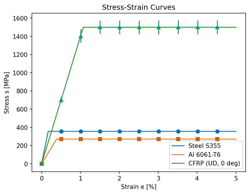
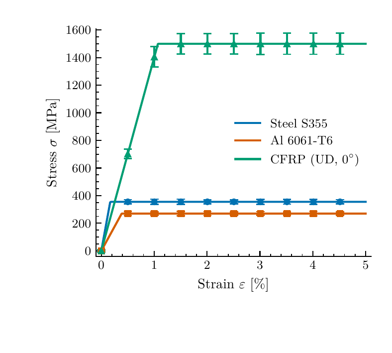
What It Looks Like in a PDF

Left: raw matplotlib defaults. Right: the same data compiled with pdflatex via PGF — what actually ends up in your paper.

Default matplotlib — DejaVu Sans, raster PNG

PGF via pdflatex — Computer Modern, same as the paper body

References

[1] Okabe & Ito (2002). Color Universal Design. jfly.uni-koeln.de/color [2] Matplotlib PGF backend: matplotlib.org/stable/users/explain/text/pgf.html [3] Hunter, J.D. (2007). Matplotlib: A 2D graphics environment. Comput. Sci. Eng., 9(3), 90–95. [4] Garrett, J.D. SciencePlots. github.com/garrettj403/SciencePlots