Mohr's circle plot for 3D stress analysis using Asymptote framework
A simple Asymptote script to plot Mohr’s Circle for 3D stress analysis. The script calculates principal stresses from a given stress tensor and draws the three Mohr’s circles along with Von Mises and Tresca stress values.
Also available on GitHub: BasemRajjoub/Mohr3D
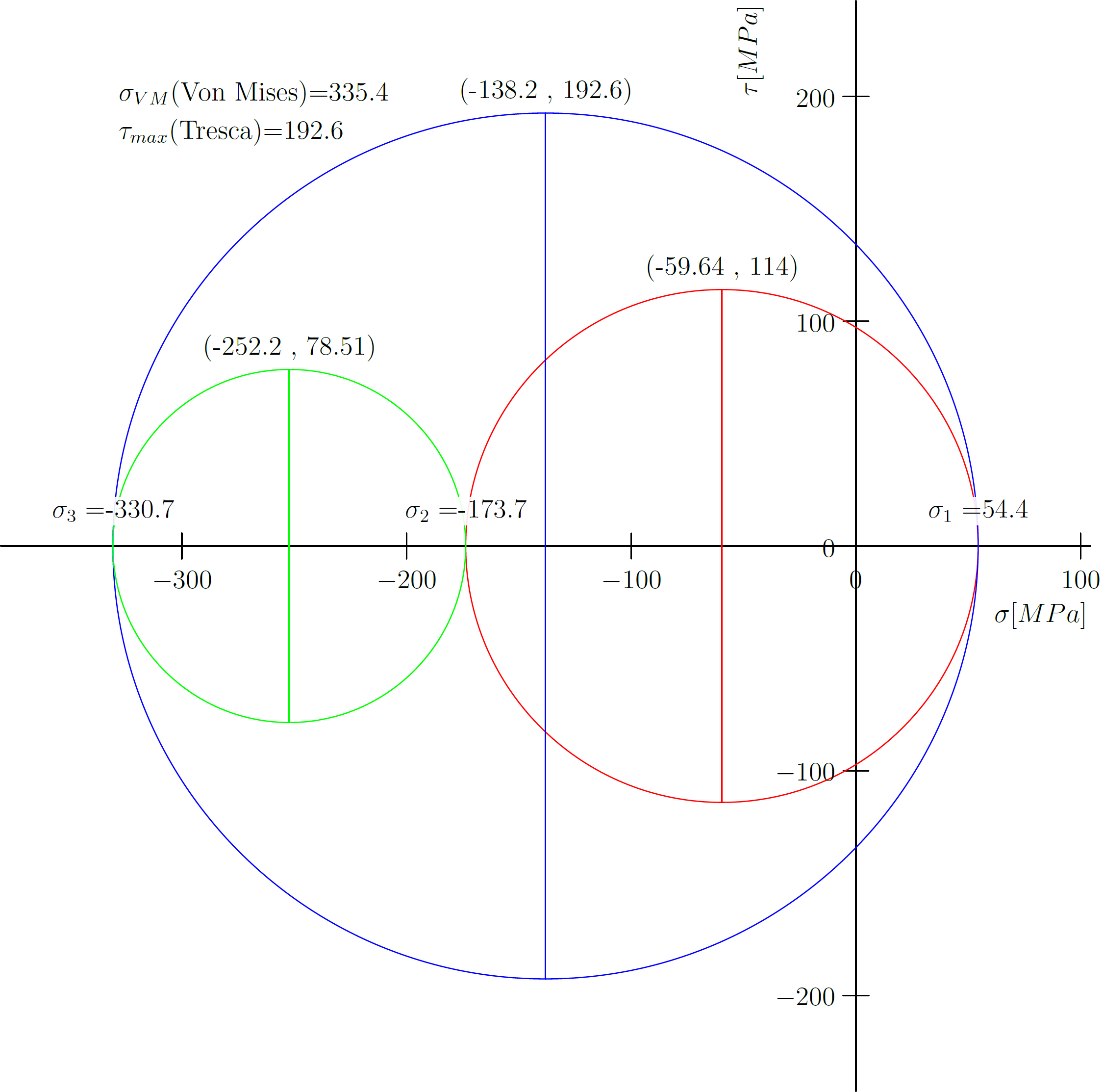 Example output: three Mohr’s circles for 3D stress state
Interactive Tool
Enter your stress tensor components below to compute principal stresses and plot Mohr’s circles live:
Code
import graph;
import settings;
settings.outformat = "pdf";

//Inputs start

string m_unit = "MPa";
real unit_step = 100;

real s_x = -100;
real s_y = -200;
real s_z = -150;
real t_xy = 50;
real t_xz = 100;
real t_yz = 150;

//Inputs end

// Stress Invariants
// https://en.wikiversity.org/wiki/Introduction_to_Elasticity/Principal_stresses

real I_1 = s_x+s_y+s_z;
real I_2 = s_x*s_y+s_y*s_z+s_z*s_x-t_xy**2-t_xz**2-t_yz**2;
real I_3 = (s_x*s_y*s_z)-s_x*t_yz**2-s_y*t_xz**2-s_z*t_xy**2+(2*t_xy*t_xz*t_yz);

real phi = (1/3)*acos((2*I_1**3-9*I_1*I_2+27*I_3)/(2*(I_1**2-3*I_2)**(3/2)));

// Principal Stresses

real s_1 = (I_1/3)+(2/3)*sqrt(I_1**2-3*I_2)*cos(phi);
real s_2 = (I_1/3)+(2/3)*sqrt(I_1**2-3*I_2)*cos(phi-2*pi/3);
real s_3 = (I_1/3)+(2/3)*sqrt(I_1**2-3*I_2)*cos(phi-4*pi/3);

// Circles

real C_1 = 0.5*(s_1+s_2);
real C_2 = 0.5*(s_1+s_3);
real C_3 = 0.5*(s_2+s_3);

real R_1 = 0.5*(s_1-s_2);
real R_2 = 0.5*(s_1-s_3);
real R_3 = 0.5*(s_2-s_3);

path c1 = circle((C_1,0),R_1);
path c2 = circle((C_2,0),R_2);
path c3 = circle((C_3,0),R_3);

draw(c1,red);
draw(c2,blue);
draw(c3,green);

draw((C_1,R_1)--(C_1,-R_1),red);
draw((C_2,R_2)--(C_2,-R_2),blue);
draw((C_3,R_3)--(C_3,-R_3),green);

xaxis(L="$\sigma ["+m_unit+"]$", axis=YZero, xmin=s_3-50, xmax=s_1+50, ticks=Ticks(Step=unit_step));
yaxis(L="$\tau ["+m_unit+"]$", axis=XZero, ymin=-R_2-50, ymax=R_2+50, ticks=Ticks(Step=unit_step));

label(L="$\sigma_1="+format(s_1)+"$", position=(s_1,0), N*3, filltype=Fill(white+opacity(0.9)));
label(L="$\sigma_2="+format(s_2)+"$", position=(s_2,0), N*3, filltype=Fill(white+opacity(0.9)));
label(L="$\sigma_3="+format(s_3)+"$", position=(s_3,0), N*3, filltype=Fill(white+opacity(0.9)));

label(L="$("+format(C_1)+"\ ,\ "+format(R_1)+")$", position=(C_1,R_1), N);
label(L="$("+format(C_2)+"\ ,\ "+format(R_2)+")$", position=(C_2,R_2), N);
label(L="$("+format(C_3)+"\ ,\ "+format(R_3)+")$", position=(C_3,R_3), N);

real s_vm = sqrt(0.5*((s_1-s_3)**2+(s_2-s_3)**2+(s_1-s_2)**2));

label(L="$\sigma_{VM}$ (Von Mises)="+format(s_vm), position=(s_3,R_2), NE);
label(L="$\tau_{max}$ (Tresca)="+format(R_2), position=(s_3,R_2), SE);
Usage
Set your stress tensor components under //Inputs start:
| Variable | Description |
|---|---|
s_x, s_y, s_z |
Normal stresses ($\sigma_x$, $\sigma_y$, $\sigma_z$) |
t_xy, t_xz, t_yz |
Shear stresses ($\tau_{xy}$, $\tau_{xz}$, $\tau_{yz}$) |
Run with: asy mohr3d.asy — outputs a PDF with the Mohr’s circle plot, principal stresses $\sigma_1$, $\sigma_2$, $\sigma_3$, Von Mises stress, and Tresca (max shear) stress.